Identify tissue structure by stCluster

In this section, we will demonstrate how to identify the organizational structure of stCluster clustering results in the spatial domain and compare it with marker genes. We will use the E2S3 slice from the MOSTA E9.5 dataset as an example.

[1]:

from st_datasets.dataset import get_data, get_mosta_data
from stCluster.run import train_and_evaluate

adata, n_cluster = get_data(get_mosta_data, id='E2S3')
adata, score = train_and_evaluate(adata, radius=2, n_cluster=n_cluster, cluster_method='mclust', cluster_score_method='ARI', ae_rate=1., adj_rate=10., pred_rate=.4)
print(score)

>>> INFO: Download dataset: 100%|██████████| 349M/349M [04:59<00:00, 1.22MB/s]

>>> INFO: dataset name: mouse organogenesis spatiotemporal transcriptomic atlas (MOSTA), section: E2S3, size: (5059, 24238), cluster: 13.(301.062s)
>>> INFO: Input size torch.Size([5059, 3000]).
>>> INFO: Graph contains 53293 edges, average 10.534 edges per node.
>>> INFO: Build graph success!
>>> INFO: Finish generate precluster embedding!
>>> INFO: Finish pre-cluster, result image is saved at "None", begin to prune graph.
>>> INFO: Finish pruning graph, result image is saved at "None".
>>> INFO: Graph contains 142757 edges, average 28.218 edges per node.
>>> INFO: Build graph success!
>>> INFO: Finish model preparations, begin to train model, input data size: (5059, 3000).

>>> INFO: Training: 100%|██████████| 1000/1000 [00:19<00:00, 51.04it/s]
R[write to console]:                    __           __
   ____ ___  _____/ /_  _______/ /_
  / __ `__ \/ ___/ / / / / ___/ __/
 / / / / / / /__/ / /_/ (__  ) /_
/_/ /_/ /_/\___/_/\__,_/____/\__/   version 5.4.10
Type 'citation("mclust")' for citing this R package in publications.

>>> INFO: Finish embedding process, total time: 31.315s.
fitting ...
  |======================================================================| 100%
{'mclust': 0.48960712924394234}

We select different hyperparameter for each slices of MOSTA datasets as follows:

slice ID	ae_rate	adj_rate	pred_rate
E1S1	0.6	0.7	0.6
E2S1	0.5	0.1	0.1
E2S2	0.4	0.3	0.6
E2S3	1.0	10.0	0.4
E2S4	0.7	0.6	0.4

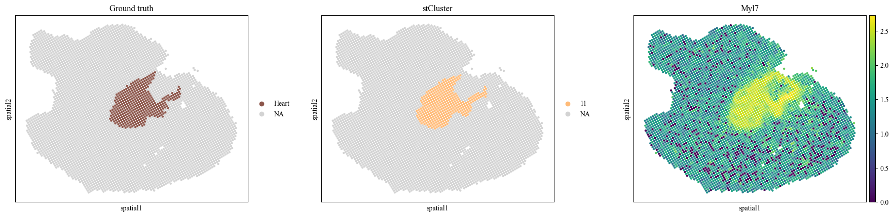
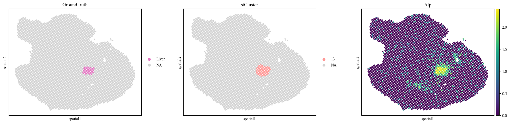
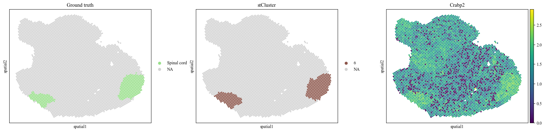
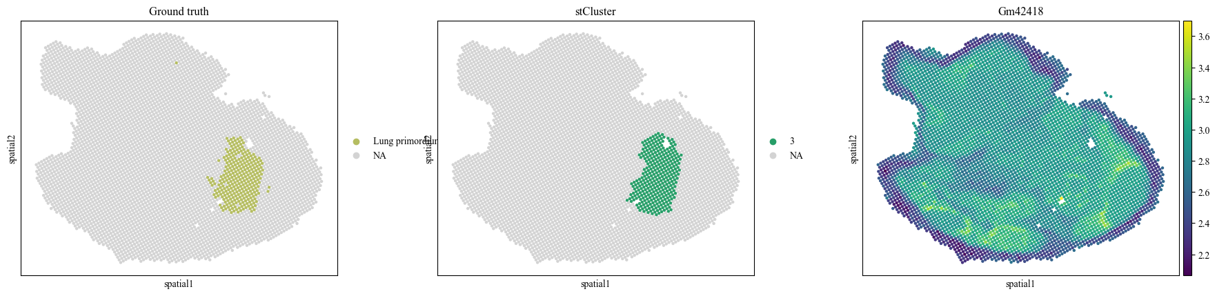
To evaluate the accuracy of our clustering result, we can compare our spatial domain distribution with the distribution of the marker genes.

Decipher domain related marker genes first:

[2]:

import scanpy as sc

sc.tl.rank_genes_groups(adata, "cluster", method="t-test", use_rep='X')
sc.pl.rank_genes_groups_heatmap(adata,  n_genes=3, groupby="cluster")

WARNING: dendrogram data not found (using key=dendrogram_cluster). Running `sc.tl.dendrogram` with default parameters. For fine tuning it is recommended to run `sc.tl.dendrogram` independently.
WARNING: You’re trying to run this on 3000 dimensions of `.X`, if you really want this, set `use_rep='X'`.
         Falling back to preprocessing with `sc.pp.pca` and default params.

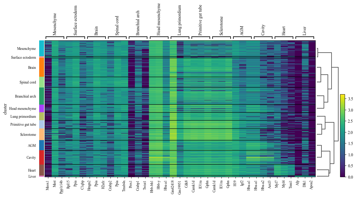
We find that gene Hmgn2, Prrx1, Myl7, Afp, Crabp2, and Gm42418 can intuitively represent the corresponding domain.

Compare those gene expressions’ distribution with our clustering result.

[3]:

sc.pl.spatial(adata, color=['cluster', 'mclust', 'Hmgn2'], spot_size=1, groups=['Brain', 9, 1], title=['Ground truth', 'stCluster', 'Hmgn2'])
sc.pl.spatial(adata, color=['cluster', 'mclust', 'Prrx1'], spot_size=1, groups=['Branchial arch', 4], title=['Ground truth', 'stCluster', 'Prrx1'])
sc.pl.spatial(adata, color=['cluster', 'mclust', 'Myl7'], spot_size=1, groups=['Heart', 11], title=['Ground truth', 'stCluster', 'Myl7'])
sc.pl.spatial(adata, color=['cluster', 'mclust', 'Afp'], spot_size=1, groups=['Liver', 13], title=['Ground truth', 'stCluster', 'Afp'])
sc.pl.spatial(adata, color=['cluster', 'mclust', 'Crabp2'], spot_size=1, groups=['Spinal cord', 6], title=['Ground truth', 'stCluster', 'Crabp2'])
sc.pl.spatial(adata, color=['cluster', 'mclust', 'Gm42418'], spot_size=1, groups=['Lung primordium', 3], title=['Ground truth', 'stCluster', 'Gm42418'])